Recently, I’ve been tasked with designing a control system for a standalone fuel supply module for alternative fuel research engines - and part of the challenge involves supplying fuel at Direct Injection system pressures to various engines under test. As a result, it was necessary to design a control system from the ground up - ultimately using LabVIEW, a NI cRIO, and a few C series modules. This write up will cover the operation of modern high pressure fuel pumps, overall system design, control system concept, and details regarding the final implementation.

Background and Operation

Nowadays, most all commonly available and used high pressure fuel pumps (HPFPs) for use in direct injection gasoline engines follow the same basic design concept. There was a time this was not the case - in the mid 2000s, there were numerous concepts being experimented with and even put into mass production, but ultimately the single piston, synchronous control style pumps as we are discussing today became the go-to for the entire industry. In fact, there are really only a few different families (and even fewer manufacturers) of these pumps in use today.

These pumps generally fall into two categories: Normally Open (NO), and Normally Closed (NC). Both operate in a mechanically similar way (the differences are primarily in relation to the electronics), but each requires a few unique control strategy considerations. The big thing to know going into this, is that these pumps must be controlled on a stroke by stroke basis - that is, the output of the pump is modulated by the duration of each stroke that the solenoid is in the pumping vs bypassing position.

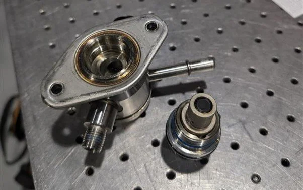
A view of the internals of a modern, single piston, high pressure fuel pump. Note that the pumps piston features a black, DLC coating to combat wear and promote sealing performance.

The Delivery Phase

The delivery phase is the portion of the pump cycle during which fuel is being delivered by the pump to the high pressure fuel system. It is almost always the case that the delivery phase, once triggered, will continue until the end of the pump stroke at TDC (Top Dead Center), and the pump piston begins to return to BDC (Bottom Dead Center). This means that varying where in the pumps cycle the Delivery Phase begin is the primary method of modulating the pumps volumetric output. This can also be referred to as Rising Edge Control (in the case of Normally Open pumps), or Falling Edge Control (in the case of Normally Closed pumps). For this write up I am using a Normally Open style pump. The angle at which delivery commences is referred to as the Start Angle (the angle from pump bottom dead center where the solenoid is enabled), and where the solenoid is switched off is referred to as End Angle. Delivery Angle is defined as the angle between the Start Angle and the End of Stroke Angle.

The Solenoid

The pumps solenoid is responsible for controlling whether (during an upwards piston stroke) the pump is in the Delivery Phase, or the Nondelivery Phase. This is typically achieved by having the solenoid control the flow of fuel between the pumps chamber and the low pressure system. Once the solenoid switches to the delivery position (closing the inlet to the chamber and allowing pressure to begin building as the piston rises), it becomes mechanically latched into the delivery position by the differential pressure present between the pumps chamber and the pump feed line. This is why the volumetric output of the pump must be controlled by varying the position of the beginning of the delivery stroke rather than the end (or both) - the solenoid would need to overcome a large amount of force, likely requiring a lot of additional energy as well as control considerations.

The Control

As with most control systems, there’s no wrong or right way to go about it. There’s a wide number of potential solutions to the problem, all with unique pros and cons. The solution can be as complex as a displacement based, linearized PID controller with numerous correction factors and feed forwards, or as simple as a bang-bang controller that either delivers a for a full stroke, or skips it entirely. You’d never guess, but I ultimately settled on the former: a displacement based controller, which includes multiplicative corrections, a feed forward, and linearization.

Feed Forwards

I love feed forwards. Maybe a bit too much given how little convincing it takes me to just characterize something and let the controller handle the transients…but this is actually a great application for them, and here’s why:

As the end result of our control is a volumetric displacement of the pump on a per cycle basis, and the engine consumes a known amount of fuel per cycle based on the operating condition, this is a perfect input to our controller, and one that will do the majority of the work with regards to pressure control. By determining the pumps piston diameter, and the profile of the pumps actuating cam, it is possible to calculate the theoretical displacement of the pump for a given delivery angle. I say theoretical because of course its not that easy, but using this relationship we can calculate the required delivery angle for the current fuel flow requirement. This’ll get us close to where we need to be, but the discrepancy in required delivery angle introduced by numerous physical factors results in the need for corrections - which brings us to the next section: corrections.

Multiplicative Corrections

Two main variables necessitate the need for a multiplicative correction factor: speed, and rail/system pressure. As rail pressure increases, the volumetric displacement of the pump tends to decrease for a given delivery angle. This can likely be mostly attributed to the increased amount of piston stroke required after the inlet valve closes before the chamber reaches system pressure and begins delivering fuel, which increases with pressure due to compressibility effects.

The second major factor, speed, has effects that are a bit more difficult to predict - but aren’t too bad to determine experimentally. Because there are multiple physical factors that contribute to the pumps change in behavior as speed varies, and this control system is designed for a specific and unique application, its unnecessary to correct for each of these physical factors individually . It is possible, but it would be quite difficult to separate each of the relevant effects in order to compensate for them individually. The primary considerations are the volumetric efficiency of the pump as a function of speed (much like an internal combustion engine, but a little bit different as a result of the reduced compressibility), and the switching time of the pump solenoid. A multiplicative correction isn’t an ideal choice for the effects due to the pump solenoid delay - but I feel its preferable over additive for a correction which is to compensate for all speed effects. Time will tell if this was a good call or not, and if it works poorly ill certainly make note of that here.

LabVIEW

For the actual impementation, I’ll be using a National Instruments cRIO9076 chassis with its integrated RT controller and FPGA, a NI9411 to read the encoder, and a TTL IO card to send the trigger signal to the solenoid power stage. An additional card for analog inputs is also used in order to read the outputs from the onboard flow meter and system pressure sensors.

The physical setup I am working with consists of a section of a camshaft from a GDI equipped engine, connected to a 15HP electric motor, powered by an external VFD. The maximum motor speed of 3450rpm correlates nicely with the maximum camshaft speed of the OEM application, but we likely won’t need to run that quickly except under specific circumstances. A Heidenhain ROD426 720ppr TTL encoder is connected to the end of the motor shaft, and is used for position determination. Initially, the Z (zero) pulse input to the system will be from the encoder, but I’ll likely switch it over to using the camshaft position sensor instead as it eliminates the need to precisely align the encoder each time the system is serviced - though potentially at the cost of some variability in the Z position cycle-to-cycle.

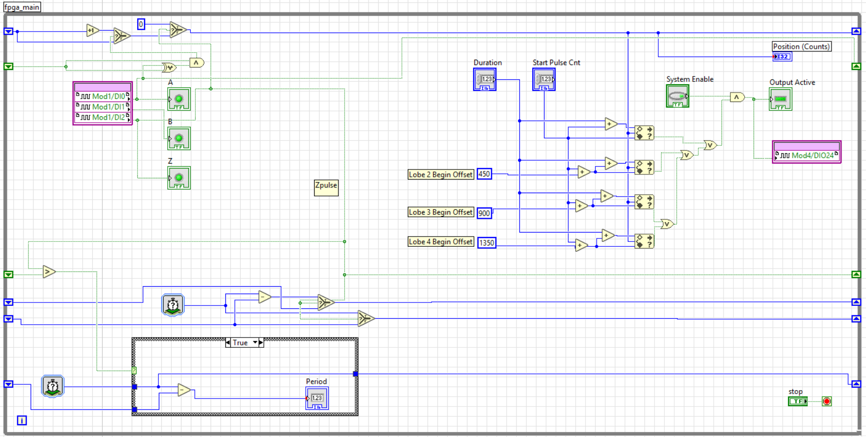
First, we’ll look at the FPGA, a Xilinx Spartan 6LX45. Due to the high number of pulses per rotation of the encoder (720) , combined with the shaft speed of 3450 rpm, the frequency of the signal we’re looking for necessitates the use of the onboard FPGA. Ultimately, all the FPGA is doing is interpreting the pulses from the encoder and determining the instantaneous shaft position, and using that information to enable or disable the solenoid output according to values being passed to it from the realtime controller. The actual control loop is implemented on the RT controller, as it offers more flexibility for additional LabVIEW functionality, and there is no need for the control loop to run on a per-cycle basis. The RT controller passes a number of parameters to the FPGA, notably: system enable signal, the number of encoder ticks after bottom dead center of each lobe where the soleonid should be enabled, and the duration (in encoder ticks) of each activation event. In the other direction, the FPGA sends current output status, flow meter input signal, pressure sensor signal, and current position back to the RT for monitoring. A very early revision of the FPGA program in LabVIEW looks as follows - though the end result will certainly be refined further:

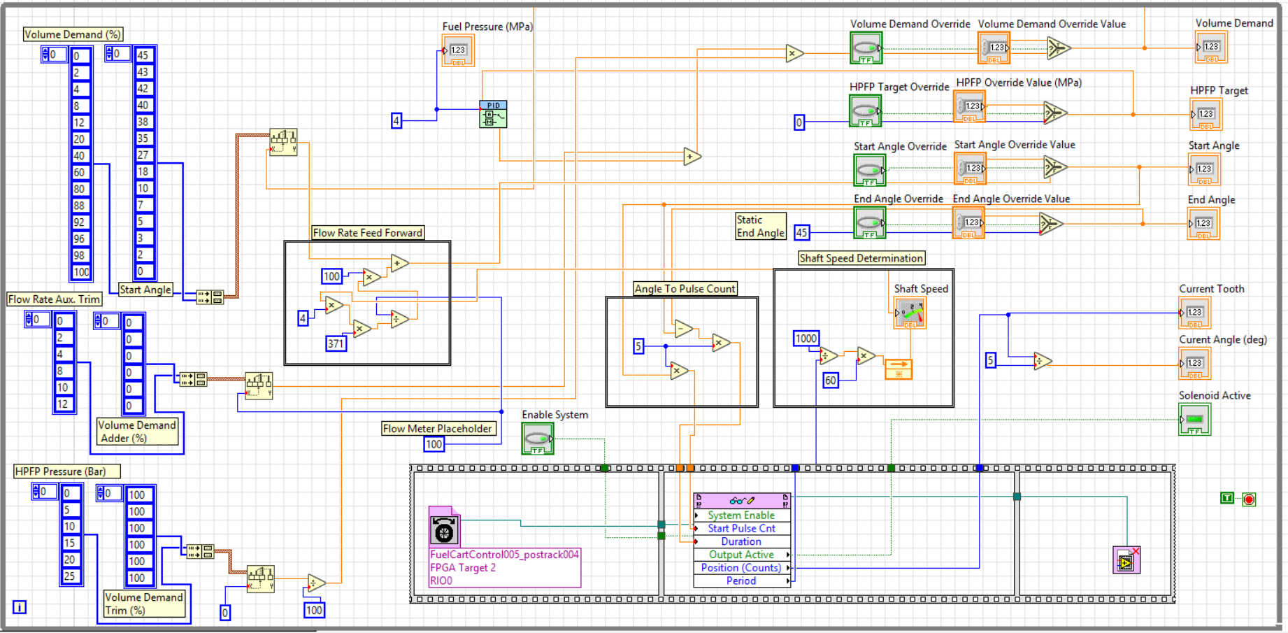
The RT Controller

As mentioned above, here in the RT controller is where the overwhelming majority of the work is happening. While the majority of this could indeed be done onboard the FPGA (albeit implemented differently), I decided to put it in the separate RT controller as I don’t know where this system may end up being used in the future, and it’s likely advantageous to not need to re-compile for the FPGA after each modification required during the initial controller design phase, and when adapting the system to new applications.

And that’s pretty much it. The end product, after all tuning and setup is done, will look a little bit different, but I expect the overall controller design to be pretty similar. There’s a lot to be done in terms of optimization - not just from a control standpoint, but also from an implementation standpoint. The method I am using to communicate control information between the RT controller and the FPGA is not great - I’m sure I’ll come across a much better way of going about this and ultimately implement that instead. Additionally, it’s likely the case that some of the feed forwards and corrections are not strictly necessary. For the most part, this controller will be dealing with engines operating at steady state, and while I’m sure a well tuned PID controller would be able to handle the majority of the control needs, I would much rather implement a controller with the theoretically needed corrections set to null, than one which requires additional work during testing and calibration.

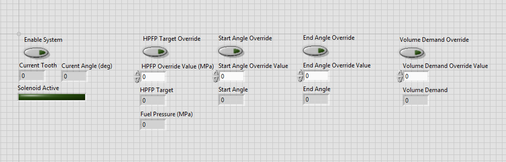
The Front Panel

Last in this section, but not least, is the front panel. This serves as the user interface - containing both control inputs such as targets, parameter overrides, and system control inputs, as well as outputs such as current pressure, start angle, PID controller output values, and more. Ultimately, once in its final form, the overwhelming majority of these parameters can be hidden since they will not be required during normal operation.

Direct Injection High Pressure Pump - Standalone Control